



To forecast demand, you must first understand what has been sold in the past. But sales history cannot be interpreted at face value. Recorded volumes depend on many factors: customer demand, product availability, price, promotions, and the distribution channel. When an item is out of stock, sales drop without demand necessarily having decreased. Conversely, a promotion can cause a one-time spike that won’t happen again.
Sales history is therefore not a forecast. It serves as the raw material from which trends, cycles, and past events can be analyzed. Its value depends less on the volume of data accumulated than on the ability to explain what each observation represents.
For retailers who manage thousands of SKUs, this distinction has direct implications for demand planning, procurement, and inventory. Misinterpreting the data can lead to overordering, stockouts, unnecessary transfers, or increased markdowns.
In this article, we’ll explore how to organize, clean, and analyze sales history data toimprove the reliability of demand forecasts and make more informed decisions.
What is a sales history?
The sales history includes transactions made over a past period. Each line typically includes a date, a product, the quantity sold, a point of sale or channel, a price, and the sales amount. Depending on the information system, other attributes may be available: discounts, promotions, returns, cancellations, inventory levels at the time of sale, supplier information, delivery times, or customer details.
Point-of-sale data tracks in-store sales, while e-commerce orders can be recorded upon confirmation, shipment, or delivery. A meaningful analysis therefore begins with a precise definition of the event being measured.
Granularity is just as important. A monthly sales total may be suitable for a fiscal year but can mask the weekly peaks that are useful for inventory planning. A daily data series reveals more variations, but at the cost of greater noise. Finally, a consolidated history by category does not allow for forecasting each product and each location. The data must be available at the level at which the decision will be made, or at a level that allows for controlled disaggregation.
Sales history and historical data: What’s the difference?
Historical data isn’t limited to sales. It can also include inventory levels, out-of-stock situations, unfilled orders, prices, promotions, returns, supplier lead times, foot traffic, the calendar, and even the weather. Sales history shows what was purchased, while the associated data helps explain the observed variations.
In particular, they help distinguish between a genuine decline in demand and a drop caused by a stockout, or between sustained growth and a one-time increase resulting from a promotion.

Why is sales history essential for demand forecasting?
Forecasting involves estimating future sales based on available information. Historical data allows us to analyze four main components: the average level of demand, its trend, its seasonality, and variations that cannot be explained by the model.
The average level provides an initial estimate. The trend indicates whether sales are increasing, decreasing, or undergoing a sustained change in pace. Seasonality highlights variations that recur on a daily, weekly, or annual basis. Finally, residual variations may result from random fluctuations, one-time events, data errors, or factors that have not been taken into account.
The weight of each component varies by product. Sales of a food product may follow a regular weekly pattern, while sales of a gardening item may depend heavily on the weather, and a replacement part may be sold on a much more irregular basis. Applying the same method to all SKUs would not allow for these differences to be taken into account.
Analyzing historical data therefore helps identify the behavior of each sales series before selecting the most appropriate forecasting method. It also makes it possible to group SKUs based on their profiles, determine the frequency of updates, and then compare the forecasts to actual sales figures.
Do past sales always reflect actual demand?
No! Sales reflect satisfied demand, not necessarily expressed demand. When the product is available and properly displayed, the gap may be small. As soon as supply constrains purchases, historical data underestimates the actual potential.
A stockout is the most obvious case. If inventory drops to zero for three days, the sales recorded over those three days do not reflect what customers would have purchased. Some of the demand is lost, while other demand shifts to a similar product, another store, or a competitor. Feeding the zero values back into the model without correction teaches the algorithm that a drop in demand has occurred, when in fact it was simply impossible to make a sale.
Other factors can cause the same discrepancy: unexpected closures, website outages, delayed search engine indexing, temporary product withdrawals, or maxed-out fulfillment capacity. Conversely, a promotion or featured listing can boost sales without permanently altering baseline demand.
Demand reconstruction involves correcting or annotating these periods. It does not mean arbitrarily replacing every outlier. It is necessary to identify the cause, estimate the unobserved volume using a documented rule, and retain the raw data to ensure traceability. This makes the forecast more reliable without erasing the product’s operational history.
What data should be linked to the sales history?
A set of quantities and dates is sufficient to create an initial statistical forecast. However, this approach has its limitations when demand is highly sensitive to business decisions or external factors. The data sources to be combined vary by industry and product, but several categories recur regularly.
Product data describes the SKU, its category, status, and lifecycle. Sales data covers pricing, promotions, and changes to the product assortment. Inventory data indicates availability, out-of-stock situations, and incoming shipments. The calendar identifies holidays, vacations, sales, and local events. Certain external factors, such as the weather, inflation, or competitors’ prices, can also influence demand.
The goal is not to connect all available databases. Each source must improve the explanation or prediction of a behavior. Adding hundreds of unreliable variables increases complexity, slows down processing, and can reduce the robustness of the models. The key criteria remain their explanatory power, their future availability, and their quality over time.
A variable that is known only after the period being forecasted cannot be used directly. Similarly, external data that is highly correlated with sales is of no value if it is not available at a frequency and over a time horizon compatible with the operational schedule.
How do you prepare a historical dataset before analyzing it?
Data preparation often requires more effort than modeling. Even a sophisticated algorithm cannot compensate for duplicate records, inconsistent dates, or data gaps treated as null values. The process must preserve a raw version, produce a corrected dataset, and document each transformation.
Harmonize the standards
Changes to item codes, store mergers, or ERP migrations often result in fragmented product lines. When old and new identifiers correspond to the same business entity, they must be reconciled. However, grouping two distinct products together simply because their descriptions are similar can create an artificial sense of continuity.
Choose a Consistent Level of Detail
Daily frequency is suitable for fast-moving products, short-term events, and frequent replenishment decisions. Weekly frequency reduces noise and makes it easier to identify trends. Monthly data is useful for an aggregated view, but is often too imprecise to effectively manage inventory.
The choice also depends on the lead time. The level of analytical detail must remain aligned with the frequency of decisions.
Handling Missing Values and Duplicates
A missing record may indicate zero sales, data that was not reported, or an inactive product. These three situations are handled differently. Duplicates, on the other hand, may result from the reimport of files or from transactions recorded in multiple systems. Correction rules must be based on the product’s status and the actual coverage of the data sources.
Identify the extreme points
An unusual volume isn’t necessarily an error. It could be due to a one-time order, a promotion, a store opening, or a local event. Automatically removing outliers deprives the model of useful information. It is better to assess them and then determine whether they are part of recurring demand, an explainable effect, or a data anomaly.
Correct data breaks and non-comparable periods
The adjustment can be based on neighboring days, the same days in previous weeks, comparable stores, or the performance of similar items. The longer the data gap, the more uncertain the estimate becomes. The adjusted value must therefore be distinguishable from an actual observed sale.
Non-comparable periods also include lockdowns, construction, major product line changes, or channel migrations. Rather than removing them, it may be appropriate to reduce their weight, isolate them using a variable, or train the model on a more representative window.

How far back should the history be retained?
There is no single “ideal” time frame that applies to all products. The depth of the historical data depends on the sales cycle, the frequency of observations, and the stability of demand. To identify annual seasonality, it is best to have several comparable years of data. For a product that has been on the market for only six months, such a long historical data set is neither available nor necessarily relevant, even when using data from a similar product.
A long-term history helps identify cycles, but it may also include patterns that no longer reflect the current situation following changes in price, distribution channel, or product mix. A shorter time frame better reflects recent trends, but places greater emphasis on one-off fluctuations.
The question, therefore, is not just how many years of data to retain, but which time periods can actually be compared. It is possible to test several time horizons and select the one that yields the most reliable forecasts. Older data can also be given less weight, particularly when using exponential smoothing.
How do you analyze sales history?
The analysis begins with a simple visualization. A time series graph organized by product and location often reveals breaks in the series, spikes, changes in levels, or cycles that are not visible in a data table. Dashboards should allow users to switch from a consolidated view to the individual data series without losing the annotations associated with specific events.
Measuring the level, dispersion, and consistency
The mean and the median provide two complementary perspectives. A significant difference between them often indicates peaks or an asymmetric distribution. The standard deviation and the coefficient of variation measure relative dispersion. The frequency of periods without sales helps identify intermittent demand.
These indicators also guide segmentation and safety stock levels. Two products with the same annual sales volume may require different policies if one sells every day and the other only through occasional orders.
Distinguishing Between Trends and Seasonality
The trend reflects the general evolution of sales over time, while seasonality refers to variations that recur at regular intervals. These might include an increase every Saturday, a spike before Christmas, or a slowdown during the summer. Seasonal coefficients are used to measure these variations, provided that they recur with sufficient consistency from one year to the next.
Decomposing the time series then makes it possible to distinguish between the level of sales, the trend, seasonality, and residual variations. This prevents an increase that is actually part of a general upward trend from being attributed to a seasonal effect. It also facilitates comparisons between different periods by neutralizing recurring variations.
Identify the explanatory factors
Correlation measures the association between two variables, but does not prove a causal relationship. A simultaneous increase in sales and traffic may indicate an acquisition effect; it may also result from a promotion that influences both. Price, discounts, availability, weather, and the calendar must be analyzed in terms of their timing and interactions.
A regression model can quantify the relationship between demand and several factors. It is useful when the variables are reliable, sufficiently variable, and available for future use. Machine learning models capture more complex relationships, but require the same precautions regarding quality, availability, and interpretation.
Segment products based on their performance
ABC segmentation classifies SKUs based on their contribution to sales or profit margin. XYZ segmentation classifies them based on their predictability or variability. Combining these approaches prevents companies from devoting the same amount of effort to a major, stable SKU, a marginal and erratic item, or a new product.
Other criteria can be used to supplement the analysis: sales frequency, product lifespan, responsiveness to promotions, seasonality, and supplier lead time. Segmentation must lead to different forecasting and management rules; otherwise, it remains merely descriptive.
Lorem ipsum dolor sit amet, consectetur adipiscing elit. Ut elit tellus, luctus nec ullamcorper mattis, pulvinar dapibus leo.
What forecasting methods should be used based on past sales?
It’s not a matter of choosing between traditional methods and artificial intelligence. The most appropriate method depends on sales patterns, the forecasting horizon, and the decisions that need to be made.
The moving average smooths out recent fluctuations and is suitable for relatively stable demand. Exponential smoothing places greater weight on the most recent observations and can account for trends and seasonality. Time series models analyze relationships between different periods, while causal approaches incorporate factors such as price, promotions, or weather. Machine learning algorithms, on the other hand, make it possible to identify more complex relationships and process a large number of time series and variables.
A complex model is not necessarily more accurate. For a short, stable time series, a simple method may yield better results. On the other hand, when forecasting demand for thousands of combinations of products and retail locations, automatic model selection becomes particularly useful. Several methods can then be tested on historical data to identify, for each time series, the one that generates the fewest errors.
Finally, a forecast should not be limited to a single figure. It must also provide an indication of its level of uncertainty, for example through a confidence interval. This information makes it possible to adjust inventory levels, compare multiple scenarios, and assess the risk associated with each decision.

How do you measure the quality of a forecast?
Comparing the forecast to actual sales helps identify errors, provided that the period under review was not affected by a disruption. Performance metrics should be selected based on their intended use and level of aggregation.
Bias indicates whether forecasts are consistently too high or too low. An absolute error measure expresses the average magnitude of the deviations. Percentages are easy to communicate, but become unreliable when actual sales are low or zero. A weighted metric may better reflect the contribution of key products.
No single KPI can fully capture the quality of the forecasting process. An acceptable average error can mask a significant underestimation of demand for priority products. Accuracy must be tracked by segment, time horizon, channel, and hierarchical level, and these results must then be linked to operational metrics: availability, out-of-stocks, excess inventory, markdowns, turnover, and capacity utilization.
The monitoring process should compare the model to a simple benchmark, such as sales from the previous period or the previous year. If an advanced solution does not outperform this baseline, its complexity is not justified. This comparison also protects against apparent improvements resulting from a change in scope.
How can you forecast demand for a new product with no sales history?
A new product may not have its own data, but that does not necessarily mean it lacks benchmarks. The forecast can use a comparable product that shares the same category, price, format, brand, channel, or launch season. The historical data for the comparable product is adjusted to account for differences in distribution, positioning, and timing.
Purchase intent, testing, pre-orders, and research data can help round out this analogy. The initial forecast, however, remains more uncertain. It should be presented as a set of scenarios—including a low, medium, and high-end scenario—and then quickly recalculated as soon as the first sales come in.
A common mistake is to maintain the pace of the first few days without taking the initial momentum into account. Another mistake is to rely on the initial analog for too long, even as the product begins to exhibit its own behavior. The system must gradually shift its weight toward the actual observations.
Is Excel sufficient for analyzing historical data?
Excel remains a useful tool for exploring a small dataset, testing a hypothesis, creating an initial visualization, or calculating a moving average. Its flexibility makes it easy to perform one-off analyses. Its limitations become apparent as the number of products, locations, channels, and recalculations increases.
A process that relies on manual copying becomes difficult to replicate and audit. Formulas may differ from one file to another, corrections are not always tracked, and the time required for processing reduces the frequency of forecasts. Consolidating multiple sources adds even more risks.
Forecasting software becomes essential when a company needs to automate data collection, clean historical data, test multiple models, manage exceptions, and distribute consistent results to the procurement team. Switching to a new tool does not eliminate the need to define business rules; rather, it makes those rules explicit, repeatable, and verifiable.
What role does artificial intelligence play in analyzing sales history?
Artificial intelligence expands the ability to process large volumes of data, incorporate exogenous variables, and detect complex relationships. It can select a model for each time series, adjust its parameters, and respond more quickly to new observations. In retail, this capability becomes crucial when forecasts involve a large number of product-location pairs.
However, it does not turn flawed data into a reliable signal. An unidentified data break, a poorly coded promotion, or an unstable reference model remains a problem, regardless of the algorithm. Machine learning can even learn the biases present in historical data more effectively.
The challenge lies in combining three elements: prepared data, tailored models, and business validation. Automation handles routine data streams, while alerts draw attention to significant deviations, changes in behavior, and key benchmarks. The human role then shifts from repetitive tasks to the analysis of exceptions and hypotheses.
How can sales history be integrated into the demand planning process?
A statistical forecast is only useful if it is incorporated into operational decisions. Demand planning makes it possible to build a baseline forecast, enrich it with available information, validate it, and then share it with the various stages of the supply chain.
The process must follow a shared schedule, with a clearly defined extraction date, forecasting horizon, update frequency, and validation rules. Business adjustments must be made in response to a specific event, such as a promotion, a product launch, or a change in distribution.
Comparing the accuracy of the statistical forecast with that of the final forecast then makes it possible to verify whether these adjustments actually improve the results. This analysis helps identify which information adds value and limit manual corrections whose usefulness has not been demonstrated.
Once validated, the forecast guides procurement, logistics capacity, transportation, and inventory targets. Discrepancies between forecast and actual volumes are then used to adjust the forecasting models and rules. Historical data is therefore not merely archived; it drives continuous improvement of the process.
What types of dashboards should be implemented?
A useful dashboard does not simply list all available metrics side by side. It should help you understand demand, monitor forecasts, and take action based on operational implications.
An initial review assesses data quality: historical coverage, missing values, detected breaks, anomalies, and the recency of the sources. A second assessment measures forecasting performance: error, bias, accuracy by time horizon, and the added value of adjustments. A third assessment links the forecast to inventory: availability, risk of stockouts, surplus, turnover, and coverage.
Exception-based monitoring is more effective than a comprehensive review. It highlights changes in levels, persistent errors, high-impact promotions, or items whose uncertainty threatens service. Thresholds must take into account the value and criticality of the product; a deviation of 20 units does not have the same impact on all batches.
Errors That Reduce the Value of Historical Data
The first mistake is to view sales as an accurate reflection of demand. The second is to correct anomalies without trying to understand their cause. Automated processing can then eliminate useful business information.
Another common mistake is aggregating data too early. A stable trend at the national level can mask very different patterns across individual stores. However, working with data series that are too detailed and contain few sales can also reduce the reliability of forecasts. It is therefore important to find the appropriate level of analysis and ensure consistency in the results across the different levels of the product-location hierarchy.
It is also risky to stick with the same forecasting method over time. A benchmark’s behavior changes over its lifecycle, depending on its distribution or competitive pressures. Models must therefore be regularly evaluated and adjusted.
Finally, statistical accuracy should not become an end in itself. A model may produce good results but still be difficult to use due to its computation time, instability, or lack of clarity. The most relevant method is the one that truly improves operational decisions.
Turning Historical Data into a Decision-Making Asset
Simply accumulating years of data is not enough to ensure reliable forecasts. If disruptions are interpreted as a decline in demand, or if promotional spikes are treated as regular sales, these errors have a direct impact on inventory, supply, and product availability.
The value of historical data therefore depends on the ability to distinguish actual sales from real demand, to explain the observed variations, and to apply a method tailored to the behavior of each product. Once validated, it allows us to identify trends, seasonality, and promotional effects, as well as to measure uncertainty and compare multiple scenarios.
Automation and predictive models make this work easier as data volumes increase. However, they do not replace data quality or business validation.
A useful sales history does more than just show what has been sold. It helps you understand lost sales, anticipate future demand, and make better decisions regarding inventory and procurement.
FAQ – Sales History
How much historical data is needed to make a forecast?
It depends on the product. A year’s worth of sales data often reveals seasonal variations, but it isn’t always enough if sales are highly irregular. For a new product, sales of similar items can help establish an initial forecast.
How can you forecast sales for a new product with no sales history?
Sales of similar products can serve as a starting point. The forecast can then incorporate the price, launch period, and planned marketing activities, and be adjusted as soon as the first sales data becomes available.
Should we use all the available years of sales data?
Not necessarily. Historical data from the past may no longer be relevant if the product mix, prices, or purchasing habits have changed. The time period selected must remain representative of the situation we are trying to forecast.
How often should forecasts be updated?
The frequency depends on the pace of sales and the decisions that need to be made. Fast-moving products or those subject to promotions require closer monitoring than stable SKUs. The key is to update the forecast early enough to be able to adjust inventory levels.